How to use data science to compare two different investments apple to apple?

An investment may make sense if we expect it to return more money than it costs. But returns are only part of the story because they are risky - there may be a range of possible outcomes. How does one compare different investments that may deliver similar results on average, but exhibit different levels of risks?

The best measure to comapre two investments apple to apple with different return and risk is Sharpe Ratio.It compares the expected returns for two investment opportunities and calculates the additional return per unit of risk an investor could obtain by choosing one over the other. In particular, it looks at the difference in returns for two investments and compares the average difference to the standard deviation (as a measure of risk) of this difference.

\[Sharpe Ratio= \frac{(R_x-R_t)}{Std R_x}\]

Where
\(R_x=\) Expected investment return
\(R_t=\) Risk free rate of return
\(Std R_x=\) Standard daviation of portfolio return

A higher Sharpe ratio means that the reward will be higher for a given amount of risk. It is common to compare a specific opportunity against a benchmark that represents an entire category of investments.

The Sharpe ratio is usually calculated for a portfolio and uses the risk-free interest rate as benchmark. The standard risk free interest rate is 3-month Treasury Bill Rate. Here, to make things easier I will consider S&P 500 as my risk free rate (Benchmark) and instead of entier portfolio I will just consider Amazon and Microsoft Share prices. you can easily find share prices online on websites like yahoo finance, google finance etc. If you want to follow along with me, you can find data here.

Lets get started now.

#Lets import all required Libraries 
import pandas as pd
import numpy as np
import matplotlib.pyplot as plt

When analyzing financial data, often its a good idea to use datatime index. You can declare that while reading your files as I am doing it over here.

#Lets read and laod required data into pandas dataframe
benchmark_data=pd.read_csv('SNP500.csv', parse_dates=['Date'], index_col=['Date']).dropna()
MSFT=pd.read_csv('MSFT.csv',parse_dates=['Date'], index_col=['Date']).dropna()
AMZN=pd.read_csv('AMZN.csv',parse_dates=['Date'], index_col=['Date']).dropna()

Lets now combine MSFT and AMZN dataframe into a single dataframe.

# Combining MSFT and AMZN into stock data
combined_data=pd.merge(MSFT,AMZN,suffixes=['_MSFT','_AMZN'],on=['Date'])
combined_data.head()

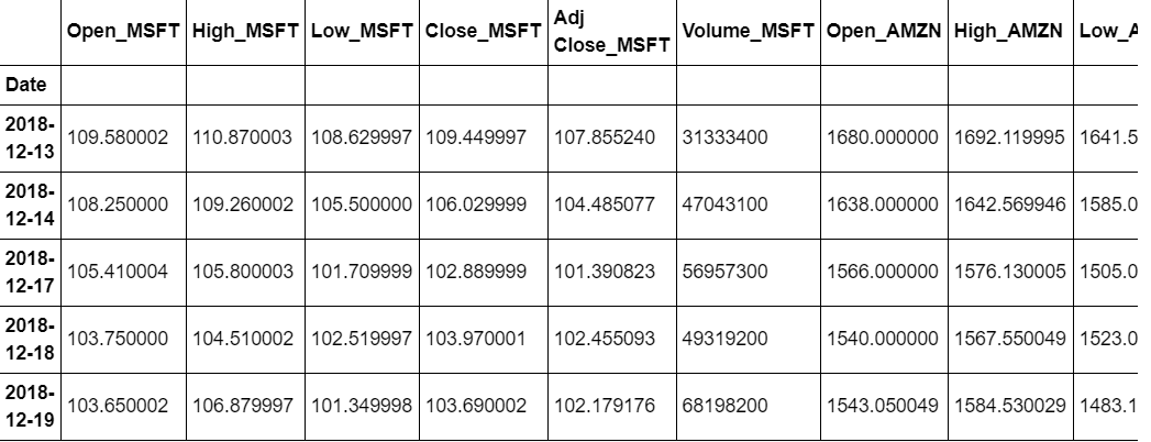
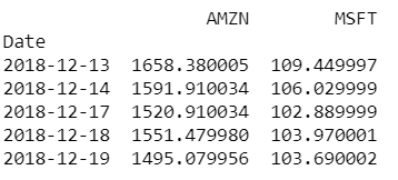
# For our analysiswe just need daily closing prices for Amazon and Microsoft, also for the benchmark.
# Stock data contains Amazon and Microsoft daily closing share prices.
stock_data=combined_data[['Close_AMZN','Close_MSFT']]
stock_data.columns=['AMZN','MSFT']
print(stock_data.head())

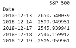
#Benchmark contains S&P 500 daily index
benchmark_data=benchmark_data[['Close']]
benchmark_data.columns=['S&P 500']
print(benchmark_data.head())

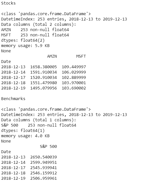
Now lets check out our data to find out how many observations we have at our disposal.

# Display summary for stock_data
print('Stocks\n')
print(stock_data.info())
print(stock_data.head())
# Display summary for benchmark_data
print('\nBenchmarks\n')
print(benchmark_data.info())
print(benchmark_data.head())

Before comparing either investment with the index of largest 500 companies in the US, let’s visualize the data, so that we’ll get better understanding about what we’re dealing with.

# visualize the stock_data
stock_data.plot(subplots=True)
plt.title('Stock Data', )
plt.show()
# summarize the stock_data
stock_data.describe()

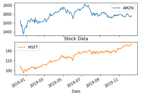
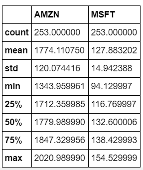
Hmm… Amazon went up 2000 mark from 1350, where as microsoft went up 150 mark from 94. What do you think was a good investment decision?\ We will see that.

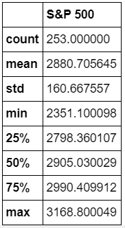
Let’s also take a closer look at the value of the S&P 500, our benchmark for the same period.

# plot the benchmark_data
benchmark_data.plot()
plt.title('S & P 500')
plt.show()

# summarize the benchmark_data
benchmark_data.describe()

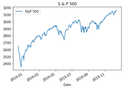
To calculate Sharepe Ratio we need returns of 2 investment opportunities under consideration, in our case return on investment for AMZN and MSFT stock.

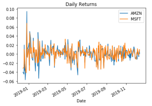
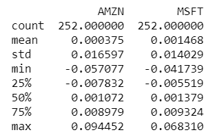
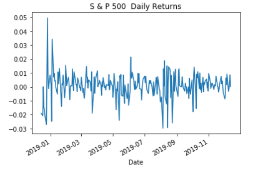
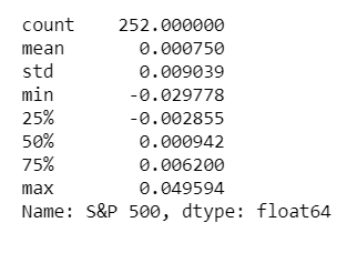
Our data shows the historical value of each investment, not the return. To calculate the return, we need to calculate the percentage change in value from one day to the next. We’ll also take a look at the summary statistics because these will become our inputs as we calculate the Sharpe Ratio.

# calculate daily stock_data returns
stock_returns = stock_data.pct_change()

# plot the daily returns
stock_returns.plot()
plt.title('Daily Returns')
plt.show()

# summarize the daily returns
print(stock_returns.describe())

# calculate daily benchmark_data returns
sp_returns = benchmark_data['S&P 500'].pct_change()

# plot the daily returns
sp_returns.plot()
plt.title('S & P 500  Daily Returns')
plt.show()

# summarize the daily returns
print(sp_returns.describe())

Now that we have daily return for each stock, we can calculate the excess return for each stock.

we need to calculate the relative performance of stocks vs. the S&P 500 benchmark. This is calculated as the difference in returns between stock_returns and sp_returns for each day.

# calculate the difference in daily returns
excess_returns = stock_returns.sub(sp_returns,axis=0)

# plot the excess_returns
excess_returns.plot()
plt.title('Excess Returns')
plt.show()

# summarize the excess_returns
print(excess_returns.describe())

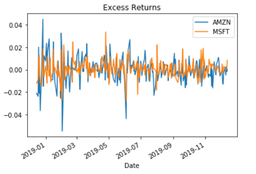
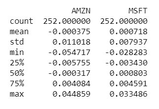
The Sharpe Ratio, Step 1: The Average Difference in Daily Returns Stocks vs S&P 500

Now we can finally start computing the Sharpe Ratio. First we need to calculate the average of the excess_returns. This tells us how much more or less the investment yields per day compared to the benchmark.

# calculate the mean of excess_returns 
avg_excess_return = excess_returns.mean()

# plot avg_excess_returns
avg_excess_return.plot.bar()
plt.title('Mean of the Return Difference')
plt.show()

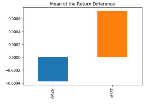
The Sharpe Ratio, Step 2: Standard Deviation of the Return Difference.

It looks like there was quite a bit of a difference between average daily returns for Amazon and Microsoft. Next, we calculate the standard deviation of the excess_returns. This shows us the amount of risk an investment in the stocks implies as compared to an investment in the S&P 500.

# calculate the standard deviations
sd_excess_return = excess_returns.std()

# plot the standard deviations
sd_excess_return.plot.bar()
plt.title('Standard Deviation of the Return Differences')
plt.show()

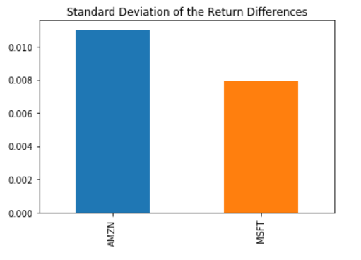
The Sharpe Ratio, Step 3: Putting it all together.

Now we just need to compute the ratio of avg_excess_returns and sd_excess_returns. The result is now finally the Sharpe ratio which indicates how much more (or less) return the investment opportunity under consideration yields per unit of risk.

The Sharpe Ratio is often annualized by multiplying it by the square root of the number of periods. We have used daily data as input, so we’ll use the square root of the number of trading days (5 days, 52 weeks, minus a few holidays): √253

# calculate the daily sharpe ratio
daily_sharpe_ratio = avg_excess_return.div(sd_excess_return)

# annualize the sharpe ratio
annual_factor = np.sqrt(253)
annual_sharpe_ratio = daily_sharpe_ratio.mul(annual_factor)

# plot the annualized sharpe ratio
annual_sharpe_ratio.plot.bar()
plt.title('Stocks vs S&P 500')
plt.show()
annual_sharpe_ratio

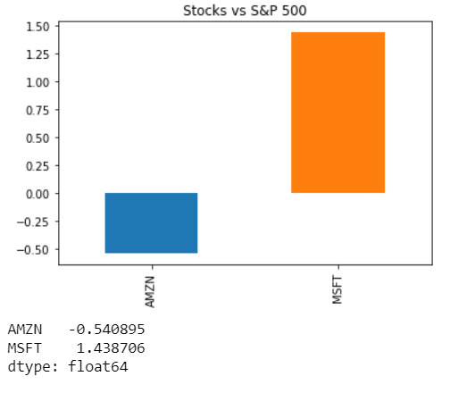
Conclusion

In 2019, Amazon had a negative Sharpe ratio as compared to Microsoft. This means that an investment in Amazon resulted less return compared to the S&P 500 for each unit of risk an investor would have assumed. This negative Sharpe Ratio here means that Risk free rate here S&P 500 performed better than Amazon stock. On the other hand, Sharpe Ratio for Microsoft was 1.43. In risk-adjusted terms, the investment in Microsoft would have been more attractive.

This difference was mostly driven by comparatively low % returns and high standard deviation of amazon over microsoft. In nutshell, investing in Microsoft would have been resulted in better returns for 2019.

Final words

When faced with investment alternatives that have both different risk and return profile, the Sharpe Ratio helps to make a decision by adjusting the returns by the differences in risk and allows an investor to compare investment opportunities on equal terms, that is, on an ‘apples-to-apples’ basis.